

Short Glossary
Animation Path
Found in the Create > Animation > Animation Path. This feature creates "path animations" where rigid body objects are forced to follow spline paths along which objects accelerate, decelerate, or undergo uniform motion according to the user's prescribed input values. This is different from simulation, in which an object's motion is determined time-step by time-step, by using Newton's laws.
Auto-ees
A data container found in the project menu in the left-side control panel. The auto-ees object controls the input parameters for simulated collisions using the Kudlich-Slibar model. Under its "defaults" menu, the user can specify the depth of penetration, coefficient-of-friction, coefficient-of-restitution, and pitch for Kudlich-Slibar collisions. Under the "object 1" and "object 2" menus, the user can access the corresponding Delta-V, pre- and post-impact speeds, pre- and post-impact yaw rates, and PDOF angles. Under the "selection" menu, the user can scroll through the various impulses that are exchanged during a simulation. Using "create user contact", the user can create a single instance of an ees object in order to modify the parameters for an individual impulse exchange. Doing this allows the user to move the impulse centroid position and enable deformation.
See:
User’s Guide | Reading Collision Data (VC5 | VC4 | VC3)
User’s Guide | Staging a Car Crash | RICSAC 1 (VC5 | VC4 | VC3)
Axles
Found in the "properties" menu in the left-side control panel. In this menu the user can add and remove axles, set the vehicle overhang, cg to front axle, wheelbase, track widths, specify tire sizes, chose between constant (default), linear, and tm-easy tire force models, set steering axles, set drive wheels, and specify suspension properties.
Damping (in “joint” menu)
Found in the “joint” menu, this is the damping coefficient for joint coupling. Every joint type, including the multibody ragdoll joint, uses a damping coefficient which helps enforce joint integrity.
Note, the damping coefficient value used internally by the simulation engine is of the form:
$$ b_{internal} = {m_{1}+m_{2} \over 1~kg} \cdot b_{user~input} $$
where \(m_{1}\) and \(m_{2}\) are the masses of the connected objects. This conversion helps ensure simulations remain stable for increases in linked object masses.
Note, if one of the connected objects is infinite in mass (using Physics > Make Unyielding / Terrain from Selection), then the internally used damping coefficient is:
$$b_{internal} = {m \over 1~kg} \cdot b_{user~input}$$
where \(m\) is the mass of the finite mass rigid body object.
Damping (in “fix orientation” menu)
Found in the “fix orientation” menu, this is the damping constant that controls the damping torque response versus articulation angle rate for a given joint.
Note, for a joint angle of articulation about the joint’s x, y, or z axis, the magnitude of the torque response is given by about the given axis is:
$$ |\tau_{damping}| = (1~m) \cdot b_{internal} \cdot (1~m) \cdot |\dot{\theta}| $$
where \(\dot{\theta}\) is articulation angle rate about the axis. An effective 1 meter lever-arm is used for internal unit conversion. Thus, we can rewrite the torque response by:
$$ |\tau_{damping}| = \tilde{b} \cdot |\dot{\theta}| $$
where \(\tilde{b}\) describes the torque response per unit change in articulation angle rate, and is given by:
$$ \tilde{b} = (1~m)^{2} \cdot b_{internal} $$
Note, the damping coefficient value used internally by the simulation engine is of the form:
$$ b_{internal} = {m_{1}+m_{2} \over 1~kg} \cdot b_{user~input} $$
where \(m_{1}\) and \(m_{2}\) are the masses of the connected objects. This conversion helps ensure simulations remain stable for increases in linked object masses.
Note, if one of the connected objects is infinite in mass (using Physics > Make Unyielding / Terrain from Selection), then the internally used damping coefficient is:
$$b_{internal} = {m \over 1~kg} \cdot b_{user~input}$$
where \(m\) is the mass of the finite mass rigid body object.
Damping (in “limits” menu)
Found in the “limits” menu, this is the spring constant that controls the torque response versus articulation angle rate, when the articulation angle is beyond the input min/max limit value for a given joint.
Note, for a joint angle of articulation about the joint’s x, y, or z axis, the magnitude of the torque response is given by about the given axis is:
$$ |\tau_{damping}| = (1~m) \cdot b_{internal} \cdot (1~m) \cdot |\dot{\theta}| $$
if \(\theta_{final} > \theta_{max}\) or \(\theta_{final}<\theta_{min}\) and 0 otherwise. Here \(\dot{\theta}\) is articulation angle rate about the axis. An effective 1 meter lever-arm is used for internal unit conversion. Thus, we can rewrite the torque response by:
$$ |\tau_{damping}| = \tilde{b} \cdot |\dot{\theta}| $$
where \(\tilde{b}\) describes the torque response per unit change in articulation angle rate, and is given by:
$$ \tilde{b} = (1~m)^{2} \cdot b_{internal} $$
Note, the damping coefficient value used internally by the simulation engine is of the form:
$$ b_{internal} = {m_{1}+m_{2} \over 1~kg} \cdot b_{user~input} $$
where \(m_{1}\) and \(m_{2}\) are the masses of the connected objects. This conversion helps ensure simulations remain stable for increases in linked object masses.
Note, if one of the connected objects is infinite in mass (using Physics > Make Unyielding / Terrain from Selection), then the internally used damping coefficient is:
$$b_{internal} = {m \over 1~kg} \cdot b_{user~input}$$
where \(m\) is the mass of the finite mass rigid body object.
Deformation Energy
Found in the Auto-EES or EES object’s contact menu. For two vehicles undergoing a contact interaction via Kudlich-Slibar impulse exchange, deformation energy is equal to the absolute value of the difference between the system’s final kinetic energy (just after impact) and initial kinetic energy (just prior to impact). Note, the system’s kinetic energy is given by the sum of linear and rotation kinetic energy terms for both vehicles.
Drawbar Length
In Virtual CRASH, drawbar length is defined as the distance between the hitch joint and the forward-most vertex of the trailer model geometry. Negative values will slide the trailer geometry forward of the joint. Positive values will slide the trailer backward of the joint.

EES
The equivalent energy speed. See the User's Guide (VC5 | VC4 | VC3) for the mathematical development of EES. Can be understood as vehicle speed resulting in a kinetic energy equal to that of the total energy lost to deformation on the vehicle. That is:
$$ E_{Loss} = {1 \over 2}\cdot m \cdot EES^2 $$
Note, the EBS, or equivalent barrier speed, is the speed at which a vehicle must collide with an infinitely massive nondeformable barrier to produce the same amount of crush damage as in the subject case. For a straight, central collision, the two can be related by:
$$ EES = EBS \cdot \sqrt{1-\epsilon^2} $$
where \(\epsilon\) is the coefficient of restitution.
Exclude overlapping
Vehicle menu found in the left-side control panel. The exclude overlapping parameters control the fraction of vertices to be excluded from the geometrical size calculations. This is useful, for example, for excluding side view mirrors from the vehicle width calculation.
Friction-body
Found in a rigid-body object's "contact" menu in the left side control panel (note, a rigid body is any object given physics attributes via "Create > Physics > Make Rigid Body From Selection". This includes vehicles). This parameter sets the upper-limit friction threshold for rigid-body object versus rigid-body object contacts. It is assumed that interacting objects will come to a common velocity at a given point-of-contact in both the normal direction, as well as the tangent direction, so long as the friction threshold value is large enough to reduce the tangent component of the closing-velocity vector to zero. If this value is too low, the system's separation velocity vector will have a non-zero tangent component at the given point-of-contact. Rigid-body objects (including multibodies) versus other rigid-body contacts use the multi-point contact model ("default-auto") to estimate the distributed impulses.
For a multibody object impacted by another rigid-body object such as a vehicle, only the multibody's friction-body value will be used by the collision model.
For two rigid-body objects (not multibodies) undergoing collision under the “default-auto” model, the friction value used for the collision will be the minimum value of the friction-body values specified for either object.
In Virtual CRASH 4, if the user transforms a multibody using the convert > "to rigid body" feature, the friction-body value used for the collision with any other object will be minimum value of the friction-body values specified for either object.
Note: by default the Kudlich-Slibar impulse-momentum model is used for vehicle versus vehicle impacts. The Kudlich-Slibar model is only enabled if both objects have "Kudlich-Slibar" selected for the preferred model in the "contact" menu.
Friction-ground
Found in a rigid-body object's "contact" menu in the left side control panel (note, a rigid body is any object given physics attributes via "Create > Physics > Make Rigid Body From Selection". This includes vehicles). This parameter sets the upper-limit friction threshold for rigid-body object versus terrain (ground) contacts. It is assumed that interacting objects will come to a common velocity at a given point-of-contact in both the normal direction, as well as the tangent direction, so long as the friction threshold value is large enough to reduce the tangent component of the closing-velocity vector to zero. If this value is too low, the system's separation velocity vector will have a non-zero tangent component at the given point-of-contact. Rigid-body objects (including multibodies) versus terrain contacts use the multi-point contact model ("default-auto") to estimate the impulses distributed over the rigid-body objects as a result of direct contact with the terrain mesh.
Hitch Overhang
In Virtual CRASH, hitch overhang is defined as the distance between the hitch joint and the rear-most vertex of the leader vehicle model geometry. Negative values will slide the joint forward of the leader vehicle’s rear-most vertex. Positive values will slide the joint backward of the leader vehicle’s rear-most vertex. Note, as the joint slides forward or backward with changing hitch overhang values, the trailer remains at a fixed position relative to the joint.
Impulse
From Newton’s Second Law, we know the total forces acting on an object is given by:
$$ \bar{F} = {d \over dt} (m \bar v) $$
The impulse, \( \bar{J} \), is given by the time integral of \( \bar{F} \):
$$ \bar{J} = \int^{t_2}_{t_1} \bar{F} (t) dt $$
where \( \bar{F} \) acts on our object during the time interval: \( t_1 \leq t \leq t_2 \).
GEV
GEV = |Delta-V|/EES. GEV is interpreted as indicating whether two vehicles will continue relative sliding motion (along the tangent plane direction) post-impact.
0.9 < GEV < 1.2 is interpreted as no post-impact sliding
0.75 < GEV < 0.9 is the start of post-impact sliding
GEV < 0.75 with post-impact sliding (like in a sideswipe)

Lock wheels
For simulated vehicle motion, "lock wheels" can be found in the "sequences" menu and is an option for all sequence types. When enabled, the "lock wheel ratio" input field will become available for each vehicle wheel. Ratio 1 corresponds to axle 1's driver-side wheel, ratio 2 to axle 1's passenger-side wheel, ratio 3 to axle 2's driver-side wheel, and so on. The ratio value represents the percent of maximum tire braking force to be applied at each time-step while the given sequence is active. The lock wheel effect begins on the integration time-step (no lag) where activated by the sequence's time or distance value. Note, for sequence “type: deceleration”, if both “lock wheels” and “wheels separately” are enabled, for wheel \(i\), the ratio used at any given time-step will be max(lock wheel ratio \(i\), wheel separate ratio \(i\)), where the wheel separate ratio \(i\) value is a function of time, brake lag, and min v. For sequence “type: acceleration” and “type: accel backward”, if both “lock wheels” and “wheels separately” are enabled for a given wheel \(i\), and the lock wheel ratio \(i\) is non-zero, then that ratio will be used to apply a braking force for that wheel.
Note: when “lock wheels” is enabled for a given sequence, the lock wheel ratios will remain active for all subsequent sequences. Lock wheels can be disengaged for a subsequent sequence by enabling “lock wheels” and typing 0 for all ratios.
Point array
Found in Create > Extended Primitives 3D > Point Array. This is a data container object primarily used for displaying total station data. Points can also be entered into a point array by hand using the "create" button. The Total Station Surface builder can be enabled by expanding the "triangulation" menu, and left-clicking on "triangulate".
Restitution-body
Found in a rigid-body object's "contact" menu in the left side control panel (note, a rigid body is any object given physics attributes via "Create > Physics > Make Rigid Body From Selection". This includes vehicles). This parameter sets the negative ratio of the normal axis projection of the separation to closing-velocity vectors for rigid-body object versus rigid-body object contacts. It is assumed that interacting objects will come to a common velocity at a given point-of-contact in the normal direction. Rigid-body objects (including multibodies) versus other rigid-body contacts use the multi-point contact model ("default-auto") to estimate the distributed impulses.
For a multibody object impacted by another rigid-body object such as a vehicle, only the multibody's restitution-body value will be used by the collision model.
For two rigid-body objects (not multibodies) undergoing collision under the “default-auto” model, the restitution value used for the collision will be the maximum value of the restitution-body values specified for either object.
In Virtual CRASH 4, if the user transforms a multibody using the convert > "to rigid body" feature, the restitution-body value used for the collision with any other object will be maximum value of the restitution-body values specified for either object.
Note: by default the Kudlich-Slibar impulse-momentum model is used for vehicle versus vehicle impacts. The Kudlich-Slibar model is only enabled if both objects have "Kudlich-Slibar" selected for the preferred model in the "contact" menu.
Restitution-ground
Found in a rigid-body object's "contact" menu in the left side control panel (note, a rigid body is any object given physics attributes via "Create > Physics > Make Rigid Body From Selection". This includes vehicles). This parameter sets the negative ratio of the normal axis projection of the separation to closing-velocity vectors for object versus terrain (ground) contacts. It is assumed that interacting objects will come to a common velocity at a given point-of-contact in the normal direction. Rigid-body objects (including multibodies) versus terrain contacts use the multi-point contact model ("default-auto") to estimate the impulses distributed over the rigid-body objects as a result of direct contact with the terrain mesh.
Sequences
For simulated vehicles, the "Sequences" menu, located under "Properties", is used to specify driver actions (steering, braking, or accelerating) or the condition of individual wheels (such as wheel lock), which typically either increases or decreases vehicle speed and steers the vehicle.
Spring (in “joint” menu)
Found in the “joint” menu, this is the spring constant for joint coupling. Every joint type, including the multibody ragdoll joint, uses a spring constant which enforces the joint integrity.
Note, the spring constant value used internally by the simulation engine is of the form:
$$ k_{internal} = {m_{1}+m_{2} \over 1~kg} \cdot k_{user~input} $$
where \(m_{1}\) and \(m_{2}\) are the masses of the connected objects. This conversion helps ensure simulations remain stable for increases in linked object masses.
Note, if one of the connected objects is infinite in mass (using Physics > Make Unyielding / Terrain from Selection), then the internally used spring constant is:
$$k_{internal} = {m \over 1~kg} \cdot k_{user~input}$$
where \(m\) is the mass of the finite mass rigid body object.
Spring (in “fix orientation” menu)
Found in the “fix orientation” menu, this is the spring constant that controls the torque response versus articulation angle beyond the initial joint articulation angle for a given joint.
Note, for a joint angle of articulation about the joint’s x, y, or z axis, the magnitude of the torque response is given by about the given axis is:
$$ |\tau_{spring}| = (1~m) \cdot k_{internal} \cdot (1~m) \cdot |(\theta_{final} - \theta_{initial})| $$
where \(\theta_{initial}\) is the initial articulation angle about the axis and \(\theta_{final}\) is the final articulation angle. An effective 1 meter lever-arm is used for internal unit conversion. Thus, we can rewrite the torque response by:
$$ |\tau_{spring}| = \tilde{k} \cdot |(\theta_{final} - \theta_{initial})| $$
where \(\tilde{k}\) describes the torque response per unit change in articulation angle, and is given by:
$$ \tilde{k} = (1~m)^{2} \cdot k_{internal} $$
Note, the spring constant value used internally by the simulation engine is of the form:
$$ k_{internal} = {m_{1}+m_{2} \over 1~kg} \cdot k_{user~input} $$
Where \(m_{1}\) and \(m_{2}\) are the masses of the connected objects. This conversion helps ensure simulations remain stable for increases in linked object masses.
Note, if one of the connected objects is infinite in mass (using Physics > Make Unyielding / Terrain from Selection), then the internally used spring constant is:
$$k_{internal} = {m \over 1~kg} \cdot k_{user~input}$$
where \(m\) is the mass of the finite mass rigid body object.
Spring (in “limits” menu)
Found in the “limits” menu, this is the spring constant that controls the torque response versus articulation angle beyond the input min/max limit value for a given joint.
Note, for a joint angle of articulation about the joint’s x, y, or z axis, the magnitude of the torque response is given by about the given axis is:
$$ |\tau_{spring}| = (1~m) \cdot k_{internal} \cdot (1~m) \cdot |(\theta_{final} - \theta_{limit})| $$
if \(\theta_{final} > \theta_{max}\) or \(\theta_{final}<\theta_{min}\) and 0 otherwise. Here \(\theta_{limit}\) is the minimum or maximum joint articulation angle limit input by the user, and \(\theta_{final}\) is the final articulation angle. An effective 1 meter lever-arm is used for internal unit conversion. Thus, we can rewrite the torque response by:
$$ |\tau_{spring}| = \tilde{k} \cdot |(\theta_{final} - \theta_{limit})| $$
where \(\tilde{k}\) describes the torque response per unit change in articulation angle, and is given by:
$$ \tilde{k} = (1~m)^{2} \cdot k_{internal} $$
Note, the spring constant value used internally by the simulation engine is of the form:
$$ k_{internal} = {m_{1}+m_{2} \over 1~kg} \cdot k_{user~input} $$
where \(m_{1}\) and \(m_{2}\) are the masses of the connected objects. This conversion helps ensure simulations remain stable for increases in linked object masses.
Note, if one of the connected objects is infinite in mass (using Physics > Make Unyielding / Terrain from Selection), then the internally used spring constant is:
$$k_{internal} = {m \over 1~kg} \cdot k_{user~input}$$
where \(m\) is the mass of the finite mass rigid body object.
Use ABS
The “use abs” option can be found in a simulated vehicle object's “braking” menu. When this option is enabled, for a given tire that has a non-zero slip angle and braking longitudinal force applied (with a non-zero ratio) simultaneously, the tire’s ratio is reduced to maintain steering control, if possible. This setting typically gives the vehicle more steering control but a reduced maximum deceleration rate.
Use Brake Curve
The “use brake curve” option models the effect of brake proportioning, such that the lock ratios for the rear wheels are reduced and the lock ratios for the front wheels are increased for a given braking sequence. The redistribution of braking force helps ensure the front wheels reach the wheel lock condition before the rear wheels.
Use ESP
The “use esp” option can be found in a simulated vehicle object’s “braking” menu. This option models the effect of an Electronic Stability Programme (ESP) or Electronic Stability Control system, which helps prevent loss of control due to oversteer events. Understeer can be corrected by manually inputting braking ratios (see below).
When “use esp” is enabled, for the given curved trajectory, at each time-step, Virtual CRASH inspects the outside front wheel and inside rear wheel to determine if the given wheel’s velocity vector local y-component (at the hub) is directed outward (away from the vehicle’s centerline). If the wheel satisfies that condition and the vehicle’s |yaw rate| exceeds the “yaw threshold” value, a braking ratio equal to the maximum value of the “efficiency” input or the user input braking ratio for the active sequence entry at that time-step is applied as an input for the tire force model for that wheel.
Note: This same behavior can be programmed manually in the sequences menu using the “lock wheels” option (for any sequence type) or “wheels separately” option (for the deceleration sequence type), where the ratios can be specified per wheel as a function of time or distance traveled. For example, in the image below, the three vehicles attempt to steer along the curved road. The yellow vehicle oversteers and loses control. The red vehicle, with “use esp” enabled, does not oversteer. The blue vehicle has manually input braking ratios for the outside front wheel to mimic the ESP performance of the red car. Both the red and blue vehicles maintain control.

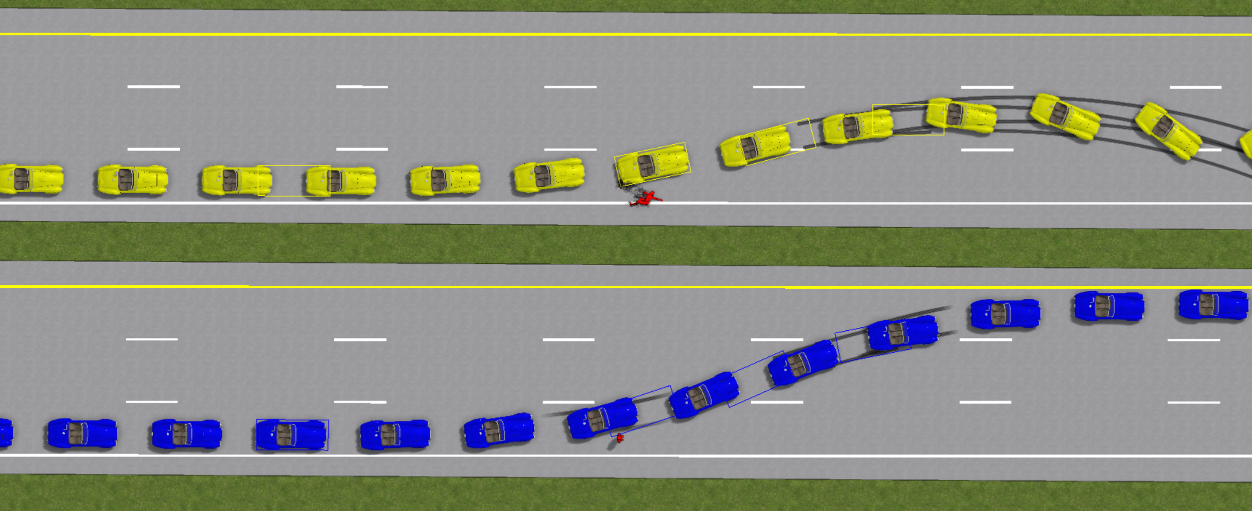
By manually programming braking ratios by wheel, you can model other ESP algorithms, including ones which correct for understeer based on yaw-rate and/or steering input thresholds of your choice. In the image below, both vehicles attempt an avoidance maneuver around the red multibody. The yellow vehicle’s sequence only includes steering inputs, while the blue vehicle includes steering inputs along with a braking ratio applied to the inside rear wheel to correct understeer, followed by a braking ratio applied to the outside front wheel to correct oversteer.
Use Pixel Center
Option used when importing orthomosaic imaging with point cloud data using a tfw (world) file. If the option is enabled, it is assumed that the tfw file(s) report the global position of the orthomosaic(s) upper-left pixel center. If the option is disabled (default option), then it is assumed the tfw(s) report the global position of the orthomosaic(s) upper-left pixel corner. Note, photogrammetry applications such as Pix4D use the pixel corner. Enabled versus disabled typically amounts a differences on the order of 5 mm in imagery positioning in global space, and therefore has minimal effect on reconstruction accuracy.
Wheels separately
For simulated vehicle motion, "wheels separately" is available in the "sequences" menu and is an option for sequence types deceleration, acceleration, and accel. backward. When enabled, the "ratio" input field becomes available for each vehicle wheel. Ratio 1 corresponds to axle 1's driver-side wheel, ratio 2 to axle 1's passenger-side wheel, ratio 3 to axle 2's driver-side wheel, and so on. The wheels separately ratio values serve the same function as “pedal position” for the given sequence type but allow the user per wheel control. Recall “pedal position” specifies the percent of maximum longitudinal tire force to be applied in the vehicle’s forward direction for sequence “type: acceleration” and backward direction for “type: accel backward”, for the vehicle’s drive wheels at each time-step where the given sequence is active. For “type: deceleration”, “pedal position” specifies the percent of maximum longitudinal tire braking force to be applied at each time-step while the given sequence is active. Similar to “pedal position”, when “wheels separately” is enabled with “type: deceleration”, a given wheel’s ratio will linearly increase from the prior sequence’s value to the new target value over a time equal to the “brake lag” input. Braking via “pedal position” or “wheels separately” ratios will engage whenever the vehicle’s speed exceeds “min v”; otherwise, it will disengage (that is, the ratios go to 0). For “type: acceleration” and “type: accel backward”, the “pedal position” or “wheels separately” ratios will engage whenever the vehicle’s speed drops below “max v” otherwise the ratios go to 0.
Note, for sequence “type: deceleration”, if both “lock wheels” and “wheels separately” are enabled, for a wheel \(i\), the ratio used at any given time-step will be the max(lock wheel ratio \(i\), wheel separate ratio \(i\)), where the wheel separate ratio \(i\) value is a function of time, brake lag, and min v. For sequence “type: acceleration” and “type: accel backward”, if both “lock wheels” and “wheels separately” are enabled for a given wheel \(i\), and the lock wheel ratio \(i\) is non-zero, then that ratio will be used to apply a braking force for that wheel.