Chapter 10 | Reading Kudlich-Slibar Impulse Data

Introduction

In this chapter, we’ll review how to interpret collision data contained in the auto-ees and ees object data containers. To make the process straightforward, we’ll work through a simple collinear and inline impact case that can be easily compared to hand calculations.

Stage a Collision

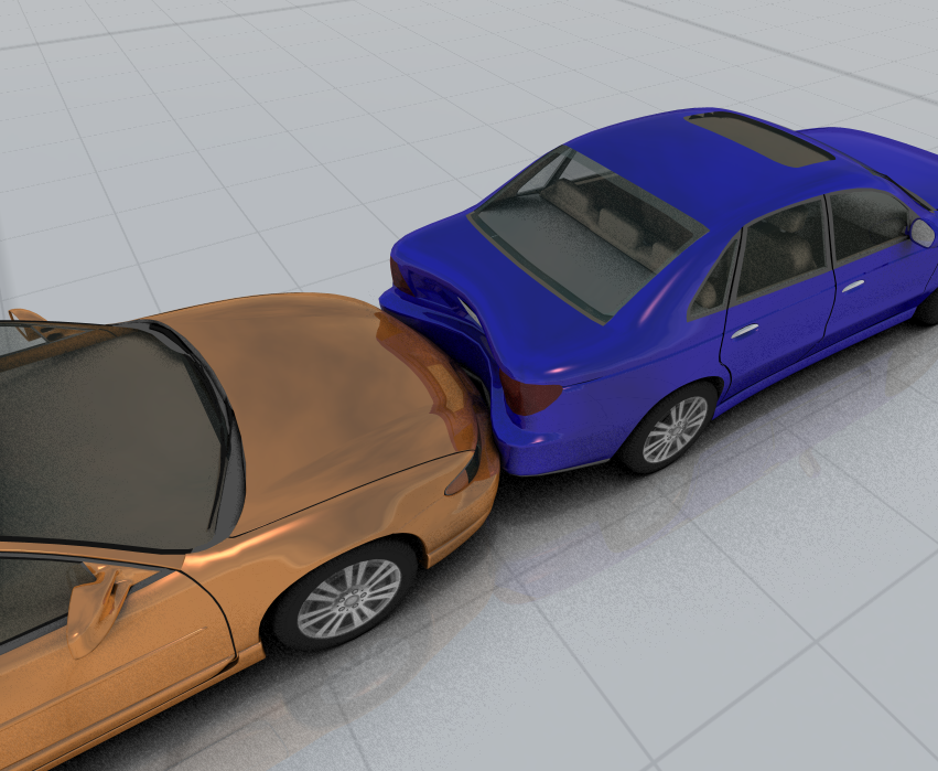
First, set up two vehicles in your Virtual CRASH environment. The figure below illustrates an inline collision between a Pontiac Grand Prix (orange) and a Saturn L300 (blue). The vehicles are positioned such that they have identical yaw orientations of 0 degrees and identical $y$ coordinates of 0 feet. The Pontiac is placed at $x$ = -10 feet and the Saturn is placed at $x$ = 10 feet. The Saturn’s initial speed is set to 5 mph, and the Pontiac’s initial speed is set to 21 mph.

As you set your vehicles’ initial speeds, you’ll notice the Virtual CRASH system immediately updates the simulation to show you the final result. Using the time slider in the lower right hand corner, you can scroll back and forward in time to isolate the moment of impact. Keep in mind that Virtual CRASH is an impulse-based simulator, which approximates impulses as being instantaneously delivered to objects undergoing collisions.

The Auto-EES Data Container

Now that you’ve set up a collision, let’s have a look at the associated collision data. Left click on “auto-ees” in the left side control panel (see below). EES objects in the left-side control panel give you direct control over the inputs to the Kudlich-Slibar impulse-momentum model, as well as allow you to instantly collect results from the model.

Next, left click on “defaults,” “misc,” and “selection” to reveal all of the auto-ees features.

Depth of Penetration

Impulse-based collision models such as Kudlich-Slibar do not rely on force–deflection relationships to resolve contact interactions. Instead, crush damage is represented through direct user input. The “depth of penetration” parameter effectively specifies the approximate total system crush. The depth of penetration, $\Delta t_{p}$, is defined in the time domain. Starting from the initial contact time $t_i$, the equal and opposite impulses are delivered to the vehicles at $ t_i + \Delta t_p $. The specific location of the impulse (force) centroid within each vehicle will be discussed later. For more information on depth of penetration, see this blog post.

Friction

The friction input value acts as a threshold. Kudlich-Slibar first solves for the impulse exchange required to bring the vehicles to a common velocity at the effective point of contact (impulse centroid). However, the tangential component of the resulting impulse vector cannot exceed the product of the input friction value and the normal impulse component. If the tangential impulse needed to fully satisfy the common-velocity condition is greater than this product, post-impact sliding contact will result. When physical evidence indicates post-impact sliding contact, lowering the friction input value can help ensure the simulation reflects this condition.

Restitution

Once the impulse calculation is completed to bring the vehicles to a common velocity and friction is accounted for, the impulse vector magnitude is increased by an amount proportional to restitution. This setting specifies the coefficient of restitution used by the collision model, with values ranging from -1 to 1. A value of 0 corresponds to a fully inelastic collision where all available collision energy is lost to inelastic effects, while a value of 1 generally corresponds to a perfectly elastic collision with no energy loss (subject to frictional effects). Negative values represent cases where the contact surfaces do not reach a common velocity, such as when components break off at the area of contact during the collision. In most vehicle collisions, realistic values typically fall between 0 and 0.5.

Pitch

Under “pitch” you will see the pitch angle of the normal axis of the collision model. This can be useful in cases of extreme front-end underride.

Select a Collision Event

In Virtual CRASH each collision event has its own associated set of collision data which is accessible through the left side control panel. To access this data, simply press “next contact” in the left side control panel beneath “selection” (see below). For simulations with multiple collision events, you can continue pressing “next contact” to cycle them all.

Once you have pressed “next contact,” you will see an impressive display in the user environment, where the impulse vectors are visible, as well as the “friction cones” (in blue) and the plane that runs orthogonal to the normal collision axis (red). You will also see a wealth of data displayed in the left side control panel which summarizes the collision event (see below). The tangent axis will be contained within this plane. The friction cone depicts the upper limit of the volume in which the impulse vector must occupy for the collision. As one decreases the allowed maximum coefficient of friction for the simulation, the size of the cone will decrease, indicating that this volume of space has also decreased. In the extreme case, where the maximum allowed coefficient of friction is set to 0, the cone will effectively enclose no volume and is represented by a line pointing along the normal axis projection, indicating that only normal impulse components will act on the vehicles.

Under “contact” you will see the magnitude of the impulse delivered to each vehicle during this event as well as the total energy lost.

Under the “defaults” section, you will find the user adjustable parameters used by the collision model. These were discussed previously above.

Left click on “object 1” and “object 2” in the left control panel to reveal the resulting values associated with this collision event.

Next, expand “position-local” and “rotation-local” to see the position of the impulse centroid and the impulse normal axis orientation.

User Defined Contacts

Scroll to the bottom of the auto-ees menu in the left side control panel. Now, left click on “create user contact.” By creating a user contact, you can modify the inputs to the collision model for this event.

Simulated Vehicle Deformation

Next, make sure your new “ees” object is selected, and scroll to the top of the new user created ees menu in the left side control panel (see below). There you will see the “deform” option disabled. Left click the box to the left of “deform” to enable simulated deformation.

Adjust Impulse Centroid Position

Now we are going to customize our impulse centroid position. This is the position in three-dimensional space at which the equal and opposite impulse vectors act on each vehicle. Click on the box to the left of “auto-position” to disable automatic positioning of the impulse vectors (see below). When Virtual CRASH automatically sets the centroid positions, it uses the overlap of the vehicle bounding boxes at the instant of momentum exchange.

Scroll down to the bottom of the ees menu in the left control panel, and you should now see the position and orientation input controls.

Let’s now adjust the $z$-position of the impulse centroid. We are going to align this $z$-position with the vehicle centers-of-gravity in order to eliminate rotational effects from our simulation (by causing the lever-arms to have 0 length). Under “position-local”, set $z$ = 1.772 feet:

Let’s shift the $x$ position of the impulse centroid at $x$ = 4 feet to simulate a case where the bullet vehicle’s front-end stiffness is much larger than the target rear-end vehicle’s stiffness. Now scroll up and set the “Depth of penetration” value to 0.06 seconds in order to exaggerate the crush damage. Note, by scrolling down the left side control panel, and left clicking on “timing,” you will see the time at which the vehicles begin to first come into contact.

As you advance your time slider forward, you’ll notice at time greater than 0.16 seconds (initial contact time) + 0.06 seconds (from depth of penetration setting), the impulses and crush damage will have been imparted to both vehicle shells.

Finally, scroll up and left click to expand “object 1” and “object 2” in the left side control panel to reveal the vehicle data for your collision event (see below). We will now analyze this data.

The Impulse

Let’s define “vehicle 1” as the Saturn (rear impacted vehicle) and “vehicle 2” as the Pontiac. In this simple inline and collinear scenario, (65) in Appendix 1 reduces to:

$$ \bar{J}_1 = -(1+\varepsilon)\left[\left(\frac{1}{\bar{m}}\right)\mathbf{1}_{3\times 3} - \mathbf{0}_{3\times 3}\right]^{-1} \cdot \bar{v}_{\text{Rel,i}}^{P} $$

or

$$\bar{J}_1 = -(1+\varepsilon)\cdot \bar{m} \cdot \bar{v}_{\text{Rel,i}}^{P} $$

where the system’s reduced mass is given by:

$$ \bar{m} = {98.95~\text{slugs} \cdot 108.68~\text{slugs} \over 98.95~\text{slugs} + 108.68~\text{slugs}} = 51.79~\text{slugs} $$ and the closing-velocity vector at impact is given by:

$$\bar{v}_{Rel,i}^P = 7.33~\text{fps}~\hat{x}- 30.80~\text{fps}~\hat{x} = -23.47~\text{fps}~\hat{x} $$

Plugging these values into our expression for impulse gives:

$$\bar{J}_1 = (1+0.1)\cdot 51.79~\text{slugs} \cdot 23.47~\text{fps}~\hat{x} = 1,336.91 ~\text{lbs-s} ~\hat{x} = 5,946.85 ~\text{N-s} ~\hat{x}$$

This is in agreement with the reported value in the contact menu.

The orientation of the impulse vector is reported as “impulse ni” (azimuth angle) and “impulse nz” (polar angle), available in both global and local frames (see this post).

Delta-V

The $|\Delta \bar{v}|$ values associated with this impulse exchange are simply given by the ratio of impulse magnitude to object mass. $|\Delta \bar{v}_1|$ is found in the “object 1” menu and $|\Delta \bar{v}_2|$ is found in the “object 2” menu. We can estimate their values by:

$$ |\Delta \bar{v}_1| = {|\bar{J}_1| \over m_1 }= {1,336.91 ~\text{lbs-s} \over 98.95~\text{slugs}} = 9.21~\text{mph} $$

$$| \Delta \bar{v}_2| = {|-\bar{J}_1| \over m_2} = {1,336.91 ~\text{lbs-s} \over 108.68~\text{slugs}} = 8.39 ~\text{mph} $$

Both of these estimates are in agreement with the values displayed in the left-side control panel.

Note: a contact interaction between vehicles may take numerous impulse exchanges to fully resolve, and therefore the $|\Delta \bar{v}|$ associated with one of potentially many impulse exchanges may not fully characterize a vehicle’s full $|\Delta \bar{v}|$. It is preferable to estimate the “cumulative” $|\Delta \bar{v}|$ using the dynamics info tool to account for multiple impulse exchanges as well as external forces acting on the vehicles during a contact interaction.

Deformation Energy

For two vehicles undergoing a contact interaction via Kudlich–Slibar impulse exchange, the deformation energy is defined as the absolute value of the difference between the system’s final kinetic energy (just after impact) and initial kinetic energy (just prior to impact).

The system’s kinetic energy is the sum of translational and rotational kinetic energy terms for both vehicles:

$$ E_{Deformation} = |KE_f - KE_i| $$

Since there is no pre- or post-impact rotation in this inline collision example, we only need to consider translational kinetic energy.

$$ KE_{1,i} = {1 \over 2}\cdot (98.95~\text{slugs})\cdot(7.33~\text{ft/s})^2 = 2,660.54~\text{ft-lbs}$$

$$ KE_{1,f} = {1 \over 2}\cdot (98.95~\text{slugs})\cdot(20.84~\text{ft/s})^2 = 21,496.35~\text{ft-lbs}$$

$$ KE_{2,i} = {1 \over 2}\cdot (108.68~\text{slugs})\cdot(30.80~\text{ft/s})^2 = 51,547.04~\text{ft-lbs}$$

$$ KE_{2,f} = {1 \over 2}\cdot (108.68~\text{slugs})\cdot(18.50~\text{ft/s})^2 = 18,593.51~\text{ft-lbs}$$

Therefore:

$$ E_{Deformation} = |(21,496.35~\text{ft-lbs} + 18,593.51~\text{ft-lbs}) - (2,660.54~\text{ft-lbs} + 51,547.04~\text{ft-lbs})| $$

$$ E_{Deformation} = 14,117.73~\text{ft-lbs} \approx 19,141~\text{J}$$

This is in agreement with the reported value in the contact menu.

Deformation

The deformation value for a given vehicle is determined by the distance between the vehicle’s bounding box and the impulse centroid position, measured along the normal collision axis. This distance is generally influenced by the depth of penetration time as well as the pre-impact orientations and positions of the vehicles. In our example, the auto-position feature of the ees object was disabled so that the centroid could be moved further into the Saturn’s rear. As a result, the Saturn shows a larger deformation value compared to the Pontiac. In typical cases, the impulse centroid and corresponding deformation estimates will be based on known crush profiles of the subject vehicles involved.

This is indeed what we see in our simulation, as the Pontiac has a deformation value of 0.059 feet and the Saturn has a deformation value of 1.396 feet.

Objects connected by joints

The Kudlich-Slibar model is used automatically for collisions between simulated vehicle objects. When vehicles are coupled by joints to other simulated objects, such as objects connected by the rope tool, or tractors being coupled to trailers, care must be taken to obtain estimates for Delta-V values. This is because the Kudlich-Slibar model will impart impulses between objects directly undergoing contact ignoring the effect of joint coupling, and joint coupling forces will be accounted for after the initial Kudlich-Slibar calculation. This means the Delta-V value displayed in the EES object for a joint coupled vehicle undergoing contact with another vehicle will not account for the additional effective mass of the connected object. In these cases, it is best to obtain cumulative Delta-V values either from the diagram tool, dynamics report data, or the dynamics info tool.

< Chapter 9 | Contents | Chapter 11 >

Chapter 10 | VC5 User's Guide