

Blog | Spring 2023 Software Update

This Spring, the Virtual CRASH team brings a HUGE update to the Virtual CRASH 5 family of users. As usual, and for almost 20 years, this update is FREE. Read on to learn more about this awesome update.
The Adaptive Driver System (ADS)
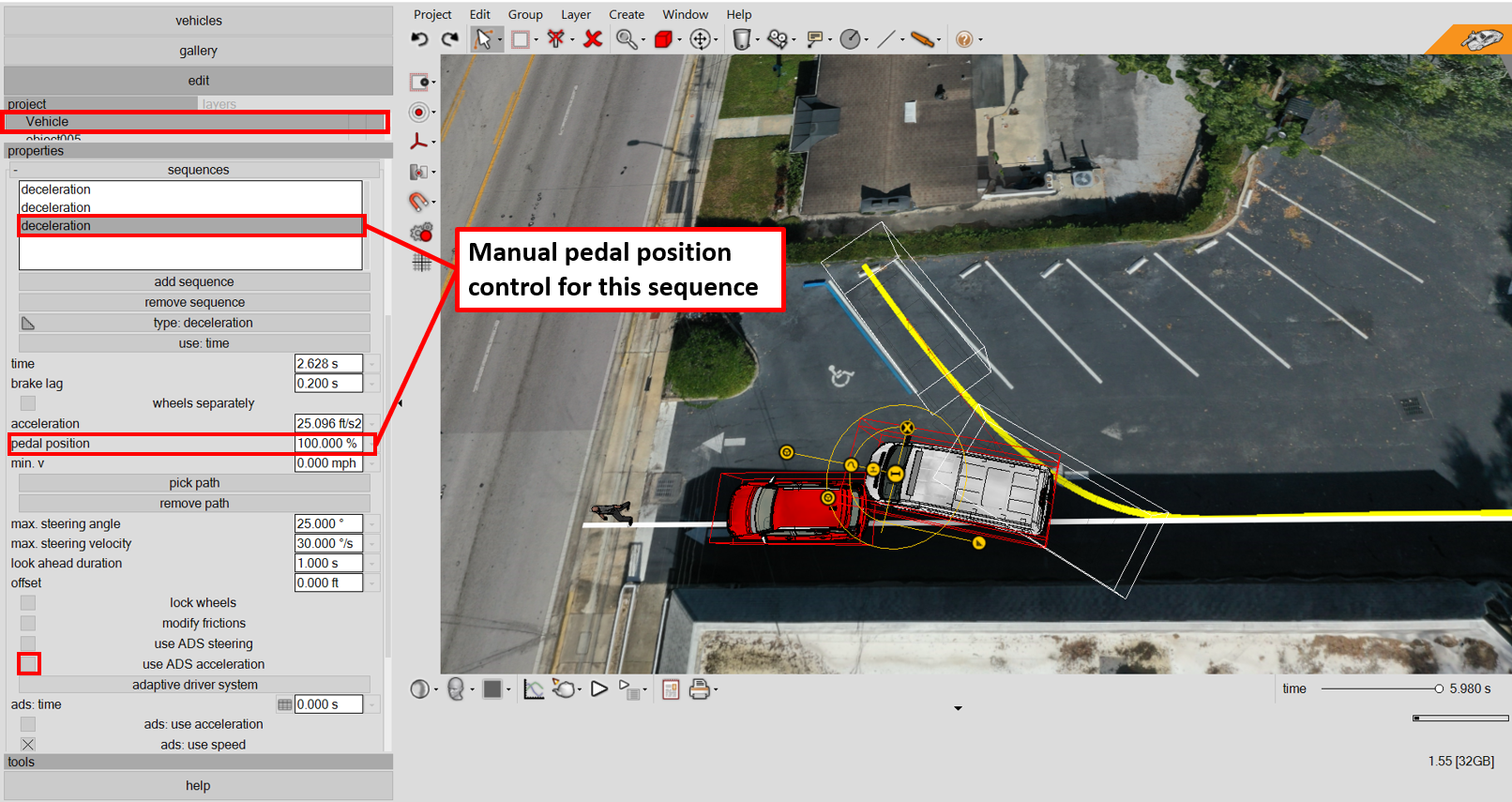
The Adaptive Driver System (or “ADS”) is an exciting new feature in Virtual CRASH 5 (also available in VC6). The ADS is a new simulation sequence controller. With the ADS, you can input acceleration or speed time-series data in tabular format, and the ADS will continuously and automatically adjust the vehicle’s pedal position to match the acceleration or speed requirements of the input data. Users can also specify time-series steering inputs in tabular form and the ADS will continuously change the vehicle steering angle to satisfy the input requirements. Before reading on, it is recommended to familiarize yourself with how sequences work in Virtual CRASH. In particular, sequences are covered in the User’s Guide (VC6 | VC5 | VC4 | VC3):
Sequences are also covered in great depth in the Simulation Basics self-paced training course: https://www.vcrashusa.com/self-paced-training-sim-basics
Note, the Advanced ADS was released as a part of the Summer 2024 Software Update. Learn more >
The typical use-cases are listed below:
Use case 1: Driving at a constant speed
If you have a vehicle traveling over complex terrain or moving with variable steering inputs, you can use the ADS to automatically increase or decrease the pedal position in order to maintain a constant speed, acting as a simple cruise control. In the figure below, we can see how the ADS can be used to maintain a constant speed. Each sequence input now has the option to give control to either steering, acceleration/deceleration pedal position, or both to the global ADS input. For each sequence input listed in the sequences menu, ADS control is indicated by the "use ADS acceleration" and "use ADS steering" toggles.
Note that if "use ADS acceleration" is enabled, the ADS acceleration (or speed) inputs will take priority over the specific sequence type's pedal position. It doesn't matter if the sequence type is deceleration, acceleration, accel. backward, uniform, or reaction, as the ADS functionality will overwrite the specific sequence type’s functionality and will automatically accelerate or decelerate the vehicle as needed to meet the user input requirements.
In the example below, we start by setting Vehicle 1’s initial speed v(t=0s) to 45 mph in the dynamics menu. We have three sequences listed in the sequences menu. The first sequence (type: deceleration) has "use ADS acceleration" enabled. This means that the first sequence's pedal position will be given by either acceleration or speed data input by the user in the "adaptive driver system" menu. In this menu, "ads: time" is set to 4 seconds in our example, indicating that the user input acceleration or speed values will control the vehicle's pedal position for simulation time from 0 to 4 seconds.


Note that "ads: use acceleration" is disabled and "ads: use speed" is enabled. This indicates that the ADS will optimize the vehicle's pedal position such that its speed stays at the value given by the "ads: speed” input, which in this case is set to 45 mph. Finally, "ads: local velocity x" is enabled, telling the ADS to optimize pedal position at each integration time-step such that the vehicle's local velocity vector x-component is 45 mph rather than the velocity vector's magnitude. If "ads: local velocity x" is disabled, the ADS will optimize pedal position such that the velocity vector's magnitude (the vehicle's speed) is equal to the "ads: speed" input value. Note, if Vehicle 1’s initial speed (v(t=0s)) is not the same as “ads: speed”, the ADS will start by applying pedal to either accelerate or decelerate the vehicle to reach a speed equal to “ads: speed” in as small a time interval as possible.
In the second sequence entry (type: uniform) for the same vehicle, we see that "use ADS acceleration" is disabled. That means that for this sequence entry, the pedal position will be set by the "pedal position" input field if the sequence type has one (note that the "uniform" sequence type does not have a pedal position input). The second sequence entry shown below has time = 4 seconds, and therefore becomes active 4 seconds after the start of the prior sequence (the prior sequence entry starts at time = 0 seconds).
Finally, a third deceleration sequence entry is introduced to apply full brakes 1 second after the start of the uniform sequence entry. Note that, again, "use ADS acceleration" is disabled. Therefore, the pedal position for this third (deceleration) sequence entry is controlled by the "pedal position" (or acceleration) input field, which in this case is set to 100%.
Using the diagram tool (https://www.vcrashusa.com/blog/2019/11/7/making-interactive-graphs), we can observe the graph (blue line) of “velocity local x” versus time for Vehicle 1. In the first region of the graph, controlled by our first sequence entry, we can see that the vehicle maintains a constant speed of 45 mph while traveling up an incline and along a slight curved trajectory (simulation time = 0 to 4 seconds). This is possible because the ADS is enabled for the first sequence, which continuously adjusts the pedal position to maintain the user input speed of 45 mph.
The second sequence entry (type: uniform) starts 4 seconds after the start of the first sequence entry, and ADS is disabled. Since uniform sequences do not have a pedal position input, we can observe a slight deceleration in the graph from time = 4 to 5 seconds. The third sequence entry begins 1 second after the start of sequence entry #2 and is of type: deceleration, again with ADS disabled. Because ADS is disabled for sequence entry #3, the pedal position is controlled by the user input field, which is set to 100% in this case. Therefore, Vehicle 1 applies full braking from time = 5 to 6 seconds. We can see an abrupt speed change in the graph due to impact after which deceleration due to braking resumes.
Below, we see the resulting ADS pedal position solution during time = 0 to 4 seconds. Also graphed is the time-average of the pedal position over this interval. Note that in some cases, depending on the complexity of the simulation, the time-average pedal position can be used to create similar simulation scenarios from manual sequence entry rather than using the ADS option. Here, we see the ADS pedal position curve change continuously in response to changing terrain and suspension forces acting on Vehicle 1.
Below we see a graph of the ADS target velocity-x value during time = 0 to 4 seconds, as well as the achieved velocity-x for Vehicle 1. Note, the difference between the two graphs is less than 0.005 mph.
The absolute value of the difference between the two graphs above is shown below by plotting “time-ADS-speed difference”.
The final crash sequence is shown in the video below:
In a similar example, the vehicle first travels downhill, then uphill, and then downhill again. A single sequence entry of type uniform is used, and ADS is enabled to maintain a constant speed of 60 mph by automatically accelerating and decelerating the vehicle as needed. The speed graph shows that the vehicle travels at around 60 mph, with some minor fluctuations. However, the ADS system maintains the target speed within 0.1 mph.
Analyzing the pedal position graph, we observe that as the vehicle travels uphill, the ADS applies mostly throttle pedal. After cresting the hill, the ADS applies mostly brake pedal. It's worth noting the impact of the "ads: accel pedal limit" and "ads: decel pedal limit" settings, both of which are set to 90% in this case. These settings can help ensure stability during steering maneuvers while the ADS is active, as the ADS may use 100% pedal, which can decrease lateral tire forces from steering input. However, reducing the pedal limits may result in not achieving the desired target speed or acceleration rate. Depending on your analysis, you may find that enabling the "use abs" and "use esp" options could be a preferable method to increase vehicle stability when the ADS is engaged. For definitions of these two options, refer to https://www.vcrashusa.com/short-glossary.
Using other options with ADS
Note in the above example, steering was controlled via the auto-driver (“pick path”) feature (https://www.vcrashusa.com/vcrash-academy-auto-driver). Just as “pick path” is available for any sequence which also uses the ADS, you may also enable “lock wheels” and “modify friction” as needed. If you do not wish to use the “pick path” feature or ADS steering (discussed below), you can also control steering using “steering time” and “steering” inputs via user input fields or the fast control icons. The ADS will also work with the various options in the “braking” menu.
Use case 2: Variable speed versus time input (with steering data)
The ADS also allows you to input time-series data for vehicle speed. The workflow is similar to the Easy EDR Animation tool, but there are some important differences to keep in mind. The ADS tool only applies force to the vehicle through pedal position inputs to accelerate or decelerate the vehicle via tire forces, whereas the Easy EDR Animation tool can be used for the same purpose, but also to model the effect of impact forces on vehicle motion. Let’s suppose we want to simulate the forward speed versus time behavior implied by the following time-series.
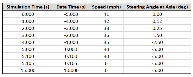
To start our simulation, we input Vehicle 1’s initial speed (v(t=0s)) into the dynamics menu as usual.
Next, we create a deceleration sequence type (again, the type is unimportant when ADS is used to control pedal position). Both “use ADS steering” and “use ADS acceleration” is used for this sequence, indicating that the ADS will control both the steering angle and acceleration/deceleration pedal position for this sequence.
Rather than entering a single value into the ads: time input field as we did in the previous example, this time we left-click on the box icon to access the dropdown menu. Next, left-click on “data”.
This will open the Diagram tool open (shown on the right in image below). Next, with our spreadsheet application open, we select the time row of your data and copy. Next, we left-click on the “paste text data”.
Now we see our data appear in the Diagram tool graph. Note, the x-axis is the row number of the input data and the y-axis is the data itself. Any of the input data values can be interactively modified using the circle grips in the Diagram tool graph or by using the input field next to the right of “value” label in the data menu area on the left side of the Diagram tool.
Notice, our pasted time data begins at -5 seconds. However, internally, time is shifted relative to the first row such that the time-series begins at simulation time = 0 seconds. Therefore, the actual time value stored in each row is irrelevant. Only the time differences (Delta-t) between a given row and the row prior to it are important.
Next, we enable “ads: use speed” to indicate we’ll be using speed data for ADS pedal position control. Then, we left-click on the “ads: speed” dropdown menu.
Next, we copy and paste our speed data into the Diagram tool.
Now we see our speed data graphed versus row number.
Note, in this example, we’ve modified the speed time-series data to force 100% braking at about simulation time = 5.1 seconds by setting speed = 0 mph. This could also be accomplished by adding a second sequence entry (with “use ADS acceleration” disabled) of type = deceleration, with pedal position = 100%, and time = 5.1 seconds.
Next, we left-click on the “ads: steering” dropdown menu and left-click on “data”.
Here again, we copy and paste our steering data into the Diagram tool.
Here we see our steering angles plotted against row number.
Here we see the resulting vehicle motion with our steering and velocity inputs specified for the ADS. We show the positions for each vehicle in 1 second increments.
Below we see the ADS target acceleration and speed graphs. When a user inputs speed data to the ADS, the average acceleration between time intervals is calculated. These accelerations are then used as targets which can be achieved via adjustments to pedal position at each time-step. Note, if “ads: local velocity x” is enabled, the ADS adjust pedal position to match the target the longitudinal acceleration vector component rather than the magnitude.
Below we see a comparison of the ADS input data and the speed and steering output from the dynamics report.

The video for this simulation is shown below.
Use case 3: Maintain constant rate of acceleration
Another use of the ADS is to maintain a constant rate of acceleration, if possible, no matter what is acting on the vehicle. In the example below, we see our tractor-tractor trailer, which begins at rest on an incline. Despite the extra weight of the trailer and the slope of the terrain, we see in the velocity graph, our tractor-trailer system achieves the desired behavior based on the target “ads: acceleration” input value. Note, just prior to impact with the vehicle down the road, we switch to a deceleration sequence entry (without ADS control). This deceleration sequence entry has a non-zero pedal position, which causes braking prior to impact. The moment where the second sequence begins can be seen in the graph below, where the blue speed curve begins to decrease. Note, the red speed curve continues increasing until time = 20 seconds (the “ads: time” input), but the “ads: acceleration” input value has no effect after the second sequence entry begins at time = 16.87 seconds.
Use case 4: Variable acceleration versus time input
In the example shown below, we once again use the ADS to control pedal position. This time however, we input an acceleration rate time-series using the “ads: time” and “ads: acceleration” dropdown menus. Simply copy from your spreadsheet application and paste into the Diagram Tool with the “paste text data” button as illustrated above for use case 2. In this example, at time = 19 seconds in the simulation, our ADS input acceleration rate goes to -5.0 ft/s^2, which is applied until time = 30 seconds. This is to trigger braking, which will only occur while speed > 0 for time > 19 seconds (since “ads: use accel. backward” is disabled). Note, another way to trigger braking is to introduce a subsequence deceleration sequence entry with time = 19 seconds.
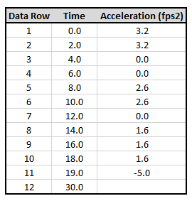
Note, as with the Easy EDR Animation tool, when using acceleration time-series data with the ADS, your data table should have N time values and N-1 acceleration values (in our example, we have 12 time values and 11 acceleration values). Acceleration is input into the ADS as a constant value over a time interval. Time intervals are determined by the progression of time values in the table’s time column. For example, acceleration[row i] is applied over a time interval of Delta-t[row i] = time[row i+1] – time[row i].
In the visualization below, we use the Path Animation tool, drawn without linking it to any vehicles. The path’s CVs are position so that it can be used as the auto-driver (pick path) path for the tractor. The same acceleration time-series data is pasted into the Easy EDR Animation feature of the animation path to provide a speed versus position graph drawn along the path itself. The “time-ADS-speed-difference” graph for the tractor indicates that the tractor’s motion matches well to the expected motion based on the acceleration time-series data. This is also verified by watching the tractor’s CG marker move relative to the animation path’s driver (blue dot).
Use case 5: Steering table
In use case 2 above, we illustrated how to import a steering table into the ADS. If you wish to input steering time-series data into the ADS without also using acceleration or speed time-series data, then simply enable the “use ADS steering” toggle for the given sequence entry and input your time-series data as needed into the “ads: time” and “ads: steering” inputs as needed. If you do not enable “use ADS acceleration” then the sequence’s acceleration or deceleration will be controlled by the sequence’s pedal position (or acceleration) input field.
Use case 6: Backward Acceleration (vehicle in reverse). Multiple sequences using the same ADS input data.
Our final use case focuses on the application of negative accelerations on vehicles using the ADS. In the example shown below, we see a van backing out of a parking space. The first sequence entry has “pick path” enabled so the van reverses while following the yellow line. ADS speed time-series data has been input, with values shown in the upper right graph. Note, negative values are used in this case, which works to apply a negative acceleration to the vehicle as long as “ads: use accel. backward” is enabled. Also note, had our vehicle started at time = 0 seconds moving in reverse (that is, value 1 in our time-series < 0 mph), we would need to set the initial speed in the dynamics menu and set vni = 180 degrees.
The second sequence entry uses the same ADS time-series data, but the “pick path” feature is switch to the white line when the van begins moving forward. In general, you can have an arbitrary number of sequences using the ADS input data to control pedal and steering. Remember, ADS speed, acceleration, and steering time-series data is always defined relative to simulation time = 0 seconds. Therefore, you will need to carefully plan the timing your sequences around the timing of the ADS time-series since the ADS time-series data is defined globally for the full simulation project.

The third sequence in this example has the ADS feature disabled when final braking is applied. Therefore, braking is controlled via the pedal position input field for this sequence. It was also possible to configure the speed input time-series data to trigger braking.
Fast shifting from reverse to drive or drive to reverse
Note, when using “ads: use accel. backward”, when the sign of the speed or acceleration input data is opposite to the vehicle’s velocity vector direction for the given time-step, the ADS will first apply brakes until speed reaches 0, then apply the opposite direction acceleration. If you have a case where you need the vehicle to switch from reverse to drive or vice versa in an abrupt manner, you will need to manually apply the corresponding sequence type without using ADS during the abrupt transition period.
Data Animation Control
Virtual CRASH 5 users can now control rigid body object motion using time-series data for (x, y, z, yaw, pitch, roll). Data can be pasted directly into the Data Animation Control tool or read from an input file. This new tool offers several applications. A few are listed below:
Virtual CRASH 5 as a production platform: If you prefer using a third-party application for physics simulation or animation motion control, you can build your project environment using Virtual CRASH 5's streamlined workflow, import your vehicles, and use time-series data from the third-party application to control vehicle motion within Virtual CRASH 5. Then, generate your final high-quality productions using Virtual CRASH 5's render engine. This new control can be used for any rigid body object, not just vehicles.
Merged visualizations: Develop multiple simulation scenarios or use Path Animation or the Momentum Solver tool to create various scenarios. Generate a dynamics report from Virtual CRASH, and paste the motion data into Data Animation Control tools linked to cloned vehicle instances. This allows you to easily superimpose multiple scenarios, as shown below.
Seamless segmented motion paths: If you prefer breaking complex scenarios into multiple, independent simulations or animations, create a unified time-series and import the complete time-series into the Data Animation Control tool to achieve seamless object motion.
Chase camera control: There are many ways to guide chase cameras in Virtual CRASH. The Data Animation Control now makes it possible to have a camera follow the exact path of your subject vehicle, but without reacting to the vehicle’s variable yaw, pitch, and roll.
The Data Animation Control workflow
In the simple example below, we start with a simulated vehicle (red) making a simple right turn. We will use this simulation to generate an example time-series dataset for use with the Data Animation Control tool. Open "Report Dynamics" and left-click "Create" to access the dynamics report.
Remember, you can simply left-click into the table and drag your mouse downward to copy from the dynamics report. Once the values are highlighted (without the header), right-click and press “copy” or press ctrl+c. This copies our data into memory.
Next, we go to Create > Animation > Data Animation Control.
Hover the mouse cursor over the (unfrozen) rigid body you would like to control with the Data Animation Control tool. The object will turn light-blue to indicate it will be selected. Next, left-click.
You will know the vehicle is linked to the Data Animation Control tool if you see the “xyz data” icon.
With the Data Animation Control tool selected, left-click on “data” under properties to see the import options.
In this example, we are going to paste the data in that we copied to memory above. Use the “data format” dropdown menu to select the appropriate format for you input data. Since we simply copied data from the dynamics report, the second option in the list is the appropriate format.
Depending on the data source, you may need to change the order in which rotations are applied. The order is defined assuming extrinsic rotations. Since Virtual CRASH applies extrinsic rotations in x-,y-, and z-axis order, we can use the default “xyz” setting. Note, there are additional options for flipping the sign of x, y, z, roll, pitch, and yaw, as well as applying offsets. These options can be modified before or after you’ve imported motion data in. We’ll leave these as the default settings as well.
Finally, left-click “paste text data” to import the data from memory.
Once the data has been imported, you should see a visual indication of the object’s motion with arrows and a blue trajectory line. The arrows provide a indication both of position and orientation at a glance (the color and arrow size attributes can be found in the “misc” menu).
Below we see the blue vehicle, controlled by the Data Animation Control tool, next to the simulation controlled red vehicle. Note, just like the Path Animation tool, when the Data Animation Control tool is used with a simulated vehicle object, you have all the standard menu options available for the simulated vehicle, such as show interpositions, sequences (to control wheel angle and rotation), geometric properties, etc.
Just like with the Path Animation tool, objects controlled by the Data Animation Control tool can interact with other rigid bodies in the scene.
If you do not want the controlled object to interact with other rigid body objects, left-click the “disable” contact toggle in the rigid body’s “contact” menu (see https://www.vcrashusa.com/blog/2022/11/1/fall-2022-software-update).
In the example below, we set up three identical environments: one with the simulated subject crash, one for the simulated alternative scenario (where defendant does not speed), and the merger of the two, where all four vehicles are controlled with Data Animation Controllers. This process was made simple by the copy-paste functionality from the dynamics report. The two simulation scenarios could also be from two different projects, where the (time,x,y,z,yaw,pitch,roll) data is saved in ASCII format and loaded into the Data Animation Control tools using the “import from file” option.
To load data from an input file, you’ll need to use one of the formats shown in the “data format” dropdown menu discussed above. Save your data in tab delimited ASCII format, like the example below, without a header.

After specifying the needed file format, and any of the other options described above, left-click on the Data Animation Control tool, then left-click “import from file”, locate your file, and left-click “open”.
You should now see the light blue arrows and a light blue trajectory line for your data.
To position the animated object in the same global position as indicated the input data (rather than an arbitrary local position), simply set reference point (x,y,z) to (0,0,0).
Note, just like with the Path Animation tool, wheel rotation and suspension effects are shown when a simulated vehicle object is controlled with the Data Animation Control tool (again rotation and steering can be customized with the Fast Control Icons or sequence entries). If you prefer using wheel data, in addition to vehicle body data, from a third-party application, then simply remove the axles from the simulated vehicle object in Virtual CRASH. Import your mesh wheels, convert them to rigid bodies, and animate each individual wheel with its own Data Animation Control.
Diagram Tool Control
The Data Animation Control allows you to inspect graphs of the (time,x,y,z,yaw,pitch,roll) input data. To see the data for one of these variables, left-click on the box to the left of the data input field and left-click the “edit” button.
You should then see the Diagram tool appear. Click on any of the variable names in the controller window on the left to see a graph of the values. Note, you can modify the values in the input fields or in the graph itself using the Diagram tool (be careful when clicking in the graph’s window).
Scrolling all the way down the “data” menu in “properties”, you’ll find the “paste text data” button, which allows you to paste data in one variable at a time.
Below we show the video for this project.
Constrained to Unconstrained Motion
At the bottom of the “data” menu, you will find the “continue with kinetics” toggle. You can use this toggle to switch your vehicle or object from constrained motion via Data Animation Control to unconstrained motion controlled with simulation. You can switch to simulation control at any moment you wish with the “start time” input.
Once the vehicle is controlled by simulation, you can use the simulation sequence menu to specify driver actions as usual.
The “continue with kinetics” feature allows users to specify pre-impact motion using third-party applications but use Virtual CRASH simulation for contact interactions and post-impact motion.
Linking
Data Animation Controls can be linked to rigid bodies. This allows for the possibility of using motion relative to a parent object as input data.
Make a Chase Camera
To create a chase camera which follows the same trajectory as your subject vehicle, first make a dummy object. This can be a vehicle from the database, or a CAD primitive such as a sphere (see below). If you use a CAD primitive shape, you’ll need to convert it to a rigid body (Create > Physics > Make Rigid Body from Selection). Once you have your dummy object in the scene, disable contact interactions by left-clicking on the “disable” toggle in the object’s “contact” menu. Next, attach a Data Animation Control tool to the object using the same workflow shown above. In the example below, we’ve attached a Data Animation Control tool to a (yellow) sphere. We then used the copy paste functionality reviewed above to make our rigid body sphere move along the exact same trajectory as the white SUV shown below (copying the SUV’s data from the dynamics report). We modified the Data Animation Control’s position-local (x,y,z) value so that there’s an offset between the SUV’s trajectory and the sphere’s. We then attached a camera target to the CG position of our SUV and attached the camera to the yellow sphere. Ultimately, you’ll hide the dummy object before production. We used the diagram tool function to modify the camera’s position-local y position as a function of time relative to the sphere for more interesting camera action.
To eliminate the effect of dummy object’s time-dependent yaw, pitch, and roll on the camera itself, use the dropdown menus to set these values to constant in the Data Animation Control tool as shown below. This ensures that the camera’s position changes versus time changes in the exact same way as the dummy object independent of the camera’s position-local value (no matter how the dummy object rotates).
Near and Far Plane Camera Clipping Control
Cameras now have near plane and far plane clipping control. Any 3D objects that fall within these two planes will be rendered. Any 3D objects between the camera in the near plane or beyond the far plane will not be rendered. This allows for the possibility of generating slices or cutaway or cross-sectional views.
In the example below, we see our vehicle partially obscured by the wall.
Here we see the same scene, but with the near plane moved further away from the camera. This has the effect of slicing out the wall so we can see our vehicle unobstructed.
The cutaway view is shown in the video below:
In the “environment” menu (deselect all objects to see this menu), you will find the near and far plane distance properties for the interactive camera view. In the example below, we see while in perspective mode, the default far plane distance is too small, causing clipping in the horizon of this large aerial image (note the image would still render in skylight or direct light).
By increasing the far plane distance value, the clipping effect is eliminated.
New Vehicle Models
This update brings VC5 users 20 new vehicles and objects.
Windows Scale Setting
VC5 user no longer need to use the “Override high DPI scaling behavior” option when scaling is used on high resolution displays (https://www.vcrashusa.com/kb-vc-article107).